Following up on my previous post, I tried the regression approach for predicting future snow depth from current values. As you recall, I produced a plot that showed how much snow we’ve had on the ground on each date at the Fairbanks Airport between 1917 and 2013. These boxplots gave us an idea of what a normal snow depth looks like on each date, but couldn’t really tell us much about what we might expect for snow depth for the rest of the winter.
Regression
I ran a linear regression analysis looking at how snow depth on November 8th relates to snow depth on November 27th and December 25th of the same year. Here’s the SQL:
SELECT * FROM (
    SELECT extract(year from dte) AS year,
        max(CASE WHEN to_char(dte, 'mm-dd') = '11-08'
                 THEN round(snwd_mm/25.4, 1)
                 ELSE NULL END) AS nov_8,
        max(CASE WHEN to_char(dte, 'mm-dd') = '11-27'
                 THEN round(snwd_mm/25.4, 1)
                 ELSE NULL END) AS nov_27,
        max(CASE WHEN to_char(dte, 'mm-dd') = '12-15'
                 THEN round(snwd_mm/25.4, 1)
                 ELSE NULL END) AS dec_25
    FROM ghcnd_pivot
    WHERE station_name = 'FAIRBANKS INTL AP'
        AND snwd_mm IS NOT NULL
    GROUP BY extract(year from dte)
    ORDER BY year
) AS sub
WHERE nov_8 IS NOT NULL
    AND nov_27 IS NOT NULL
    AND dec_25 IS NOT NULL;
I’m grouping on year, then grabbing the snow depth for the three dates of interest. I would have liked to include dates in January and February in order to see how the relationship weakens as the winter progresses, but that’s a lot more complicated because then we are comparing the dates from one year to the next and the grouping I used in the query above wouldn’t work.
One note on this analysis: linear regression has a bunch of assumptions that need to be met before considering the analysis to be valid. One of these assumptions is that observations are independent from one another, which is problematic in this case because snow depth is a cumulative statistic; the depth tomorrow is necessarily related to the depth of the snow today (snow depth tomorrow = snow depth today + snowfall). Whether it’s necessarily related to the depth of the snow a month from now is less certain, and I’m making the possibly dubious assumption that autocorrelation disappears when the time interval between observations is longer than a few weeks.
Results
Here are the results comparing the snow depth on November 8th to November 27th:
> reg <- lm(data=results, nov_27 ~ nov_8)
> summary(reg)

Call:
lm(formula = nov_27 ~ nov_8, data = results)

Residuals:
    Min      1Q  Median      3Q     Max
-8.7132 -3.0490 -0.6063  1.7258 23.8403

Coefficients:
            Estimate Std. Error t value Pr(>|t|)
(Intercept)   3.1635     0.9707   3.259   0.0016 **
nov_8         1.1107     0.1420   7.820 1.15e-11 ***
---
Signif. codes:  0 ‘***’ 0.001 ‘**’ 0.01 ‘*’ 0.05 ‘.’ 0.1 ‘ ’ 1

Residual standard error: 4.775 on 87 degrees of freedom
Multiple R-squared:  0.4128,    Adjusted R-squared:  0.406
F-statistic: 61.16 on 1 and 87 DF,  p-value: 1.146e-11
And between November 8th and December 25th:
> reg <- lm(data=results, dec_25 ~ nov_8)
> summary(reg)

Call:
lm(formula = dec_25 ~ nov_8, data = results)

Residuals:
    Min      1Q  Median      3Q     Max
-10.209  -3.195  -1.195   2.781  10.791

Coefficients:
            Estimate Std. Error t value Pr(>|t|)
(Intercept)   6.2227     0.8723   7.133 2.75e-10 ***
nov_8         0.9965     0.1276   7.807 1.22e-11 ***
---
Signif. codes:  0 ‘***’ 0.001 ‘**’ 0.01 ‘*’ 0.05 ‘.’ 0.1 ‘ ’ 1

Residual standard error: 4.292 on 87 degrees of freedom
Multiple R-squared:  0.412,     Adjusted R-squared:  0.4052
F-statistic: 60.95 on 1 and 87 DF,  p-value: 1.219e-11
Both regressions are very similar. The coefficients and the overall model are both very significant, and the R² value indicates that in each case, the snow depth on November 8th explains about 40% of the variation in the snow depth on the later date. The amount of variation explained hardly changes at all, despite almost a month difference between the two analyses.
Here's a plot of the relationship between today’s date and Christmas (PDF version)
The blue line is the linear regression model.
Conclusions
For 2014, we’ve got 2 inches of snow on the ground on November 8th. The models predict we’ll have 5.4 inches on November 27th and 8 inches on December 25th. That isn’t great, but keep in mind that even though the relationship is quite strong, it explains less than half of the variation in the data, which means that it’s quite possible we will have a lot more, or less. Looking back at the plot, you can see that for all the years where we had two inches of snow on November 8th, we had between five and fifteen inches of snow in that same year on December 25th. I’m certainly hoping we’re closer to fifteen.
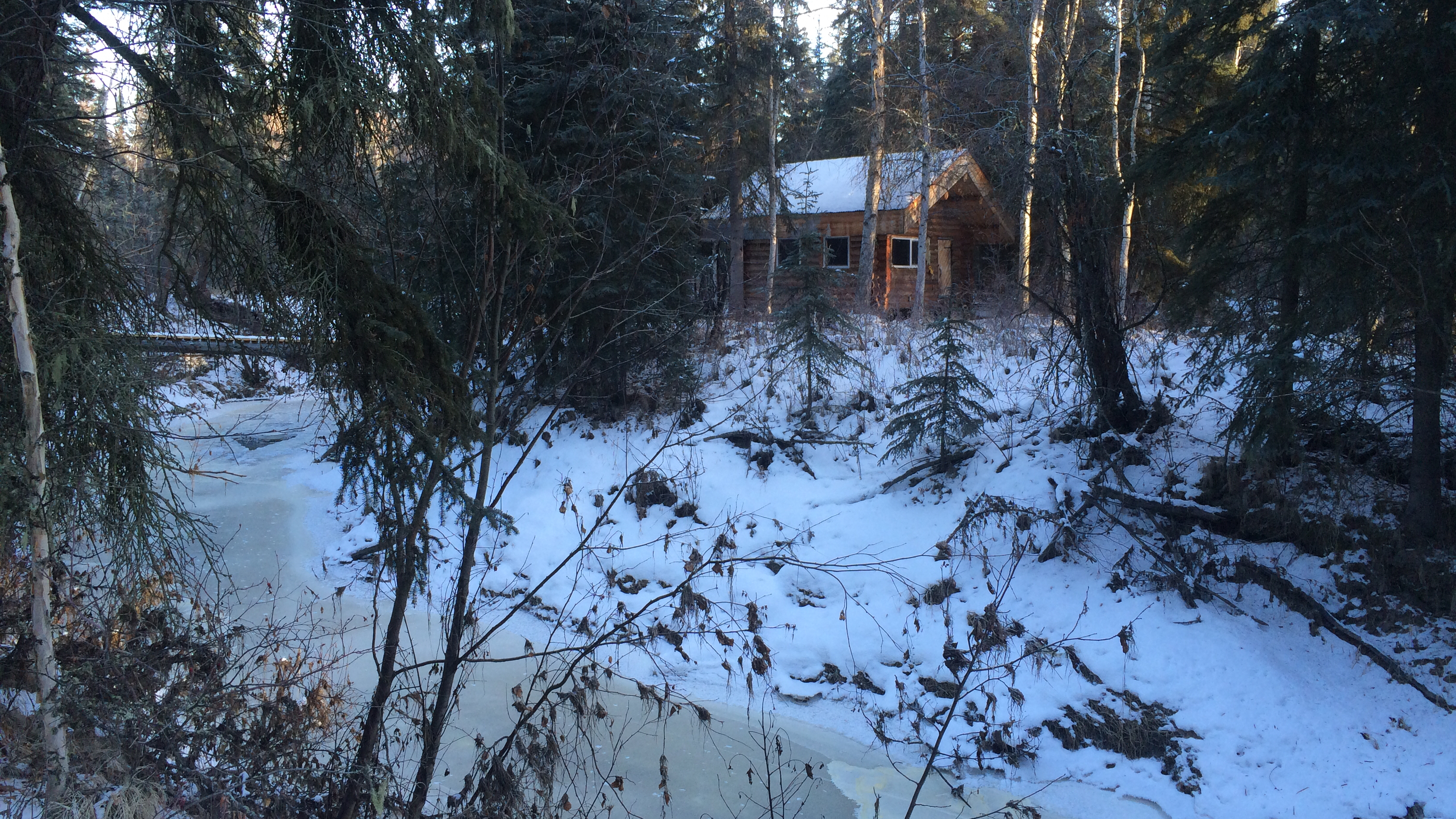
bridge and back cabin, low snow
Winter started off very early this year with the first snow falling on October 4th and 5th, setting a two inch base several weeks earlier than normal. Since then, we’ve had only two days with more than a trace of snow.
This seems to be a common pattern in Fairbanks. After the first snowfall and the establishment of a thin snowpack on the ground, we all get excited for winter and expect the early snow to continue to build, filling the holes in the trails and starting the skiing, mushing and winter fat biking season. Then, nothing.
Analysis
I decided to take a quick look at the pattern of snow depth at the Fairbanks Airport station to see how uncommon it is to only have two inches of snow this late in the winter (November 8th at this writing). The plot below shows all of the snow depth data between November and April for the airport station, displayed as box and whisker plots.
Here’s the SQL:
SELECT extract(year from dte) AS year,
       extract(month from dte) AS month,
       to_char(dte, 'MM-DD') AS mmdd,
       round(snwd_mm/25.4, 1) AS inches
FROM ghcnd_pivot
WHERE station_name = 'FAIRBANKS INTL AP'
    AND snwd_mm IS NOT NULL
    AND (extract(month from dte) BETWEEN 11 AND 12
         OR extract(month from dte) BETWEEN 1 AND 4);
If you’re interested in the code that produces the plot, it’s at the bottom of the post. If the plot doesn’t show up in your browser or you want a copy for printing, here’s a link to the PDF version.
Box and whisker plots
For those unfamiliar with these, they’re a good way to evaluate the range of data grouped by some categorical variable (date, in our case) along with details about the expected values and possible extremes. The upper and lower limit of each box show the ranges where 25—75% of the data fall, meaning that half of all observed values are within this box for each date. For example, on today’s date, November 8th, half of all snow depth values for the period in question fell between four and eight inches. Our current snow depth of two inches falls below this range, so we can say that only having two inches of snow on the ground happens in less than 25% of the time.
The horizontal line near the middle of the box is the median of all observations for that date. Median is shown instead of average / mean because extreme values can skew the mean, so a median will often be more representative of the most likely value. For today’s date, the median snow depth is five inches. That’s what we’d expect to see on the ground now.
The vertical lines extending above and below the boxes show the points that are within 1.5 times the range of the boxes. These lines represent the values from the data outside the most likely, but not very unusual. If you scan across the November to December portion of the plot, you can see that the lower whisker touches zero for most of the period, but starting on December 26th, it rises above zero and doesn’t return until the spring. That means that there have been years where there was no snow on the ground on Christmas. Ouch.
The dots beyond the whiskers are outliers; observations so far from what is normal that they’re exceptional and not likely to be repeated. On this plot, most of these outliers are probably from one or two exceptional years where we got a ton of snow. Some of those outliers are pretty incredible; consider having two and a half feet of snow on the ground at the end of April, for example.
Conclusion
The conclusion I’d draw from comparing our current snow depth of two inches against the boxplots is that it is somewhat unusual to have this little snow on the ground, but that it’s not exceptional. It wouldn’t be unusual to have no snow on the ground.
Looking forward, we would normally expect to have a foot of snow on the ground by mid-December, and I’m certainly hoping that happens this year. But despite the probabilities shown on this plot it can’t say how likely that is when we know that there’s only two inches on the ground now. One downside to boxplots in an analysis like this is that the independent variable (date) is categorical, and the plot doesn’t have anything to say about how the values on one day relate to the values on the next day or any date in the future. One might expect, for example, that a low snow depth on November 8th means it’s more likely we’ll also have a low snow depth on December 25th, but this data can’t offer evidence on that question. It only shows us what each day’s pattern of snow depth is expected to be on it’s own.
Bayesian analysis, “given a snow depth of two inches on November 8th, what is the likelihood of normal snow depth on December 25th”, might be a good approach for further investigation. Or a more traditional regression analysis examining the relationship between snow depth on one date against snow depth on another.
Appendix: R Code
library(RPostgreSQL)
library(ggplot2)
library(scales)
library(gtable)

# Build plot "table"
make_gt <- function(nd, jf, ma) {
    gt1 <- ggplot_gtable(ggplot_build(nd))
    gt2 <- ggplot_gtable(ggplot_build(jf))
    gt3 <- ggplot_gtable(ggplot_build(ma))
    max_width <- unit.pmax(gt1$widths[2:3], gt2$widths[2:3], gt3$widths[2:3])
    gt1$widths[2:3] <- max_width
    gt2$widths[2:3] <- max_width
    gt3$widths[2:3] <- max_width
    gt <- gtable(widths = unit(c(11), "in"), heights = unit(c(3, 3, 3), "in"))
    gt <- gtable_add_grob(gt, gt1, 1, 1)
    gt <- gtable_add_grob(gt, gt2, 2, 1)
    gt <- gtable_add_grob(gt, gt3, 3, 1)

    gt
}

drv <- dbDriver("PostgreSQL")
con <- dbConnect(drv, dbname="DBNAME")
results <- dbGetQuery(con,
                      "SELECT extract(year from dte) AS year,
                              extract(month from dte) AS month,
                              to_char(dte, 'MM-DD') AS mmdd,
                              round(snwd_mm/25.4, 1) AS inches
                       FROM ghcnd_pivot
                       WHERE station_name = 'FAIRBANKS INTL AP'
                           AND snwd_mm IS NOT NULL
                           AND (extract(month from dte) BETWEEN 11 AND 12
                                OR extract(month from dte) BETWEEN 1 AND 4);")
results$mmdd <- as.factor(results$mmdd)
# NOV DEC
nd <- ggplot(data=subset(results, month == 11 | month == 12), aes(x=mmdd, y=inches)) +
    geom_boxplot() +
    theme_bw() +
    theme(axis.title.x = element_blank()) +
    theme(plot.margin = unit(c(1, 1, 0, 0.5), 'lines')) +
    # scale_x_discrete(name="Date (mm-dd)") +
    scale_y_discrete(name="Snow depth (inches)", breaks=pretty_breaks(n=10)) +
    theme(axis.text.x = element_text(angle = 45, hjust = 1)) +
    ggtitle('Snow depth by date, Fairbanks Airport, 1917-2013')
# JAN FEB
jf <- ggplot(data=subset(results, month == 1 | month == 2), aes(x=mmdd, y=inches)) +
    geom_boxplot() +
    theme_bw() +
    theme(axis.title.x = element_blank()) +
    theme(plot.margin = unit(c(0, 1, 0, 0.5), 'lines')) +
    # scale_x_discrete(name="Date (mm-dd)") +
    scale_y_discrete(name="Snow depth (inches)", breaks=pretty_breaks(n=10)) +
    theme(axis.text.x = element_text(angle = 45, hjust = 1)) # +
    # ggtitle('Snowdepth by date, Fairbanks Airport, 1917-2013')
# MAR APR
ma <- ggplot(data=subset(results, month == 3 | month == 4), aes(x=mmdd, y=inches)) +
    geom_boxplot() +
    theme_bw() +
    theme(plot.margin = unit(c(0, 1, 1, 0.5), 'lines')) +
    scale_x_discrete(name="Date (mm-dd)") +
    scale_y_discrete(name="Snow depth (inches)", breaks=pretty_breaks(n=10)) +
    theme(axis.text.x = element_text(angle = 45, hjust = 1)) # +
    # ggtitle('Snowdepth by date, Fairbanks Airport, 1917-2013')

gt <- make_gt(nd, jf, ma)
svg("snowdepth_boxplots.svg", width=11, height=9)
grid.newpage()
grid.draw(gt)
dev.off()